Seven Simple Tips To Win Your Excel Battle

By Aliya Khayat, Energy Billing & Settlement Clerk

Have you ever sat there in front of your computer deleting blank cells one by one? Were you annoyed by the feeling that this could be done in a smarter and quicker way than half an hour of you clicking? If you have ever been there, keep reading. These seven simple tricks will give you a W for this round of your daily Excel battle.

In order to see the screengrabs in a larger resolution, please download the images to your computer.

1.    Deleting blank cells/rows
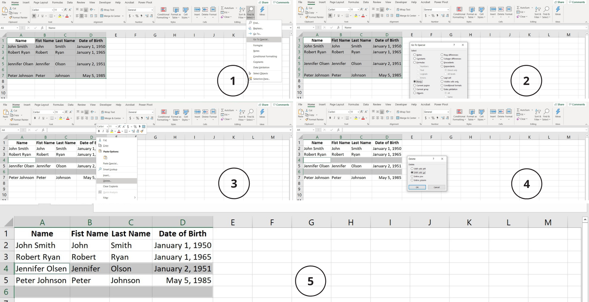
Step 1: select a list or a table where to want to delete blanks from
Step 2: click on Home => Find & Select=> Go to Special and then select Blanks in a pop-up menu
Step 3: you will see blank cells in the identified area of a spreadsheet being selected. Right-click your mouse and click Delete.
Step 4: select how you want your blank cells to disappear. In this case I selected “shift cells up”.

Viola! – the blank cells are gone. Remember, when you delete cells, data shifts within the table. If you have random blank cells, ensure that at step 4 you correctly select where you want your cells to shift.

2.    Removing duplicates
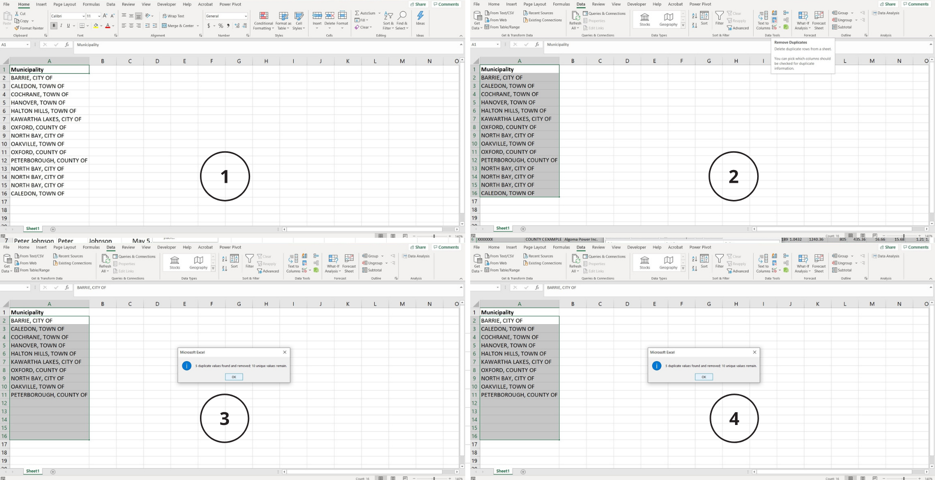
What if you are seeing duplicate values that you need to get rid of?  Say you have a list of Ontario municipalities and you need to count all unique values. Those nasty duplicates can be particularly annoying. Here’s what you can do.

Step 1: select a list or a table where to want to remove duplicate values from
Step 2: click on the Data tab at the top => look for a magic symbol 
Step 3: after you clicked on the magic symbol you can select in a pop-up menu which columns you want duplicates to be removed from. In this case we have only one column.
Step 4: click Ok

Mr. Excel will let you know how many duplicates it deleted and how many unique municipalities were left on that list.

“Whoa, too fast. What if I want to see the duplicates?”. That’s a fair point. Let’s learn how to highlight those duplicate or unique data entries.

3.    Conditional formatting to highlight duplicate or unique data values 
If you have a list or table with duplicate values conditional formatting is a great helper to highlight those duplicate or unique values. Please remember that if there are spaces or any other differences in those data values, conditional formatting won’t consider them duplicated.

Let’s go back to our original list of municipalities.

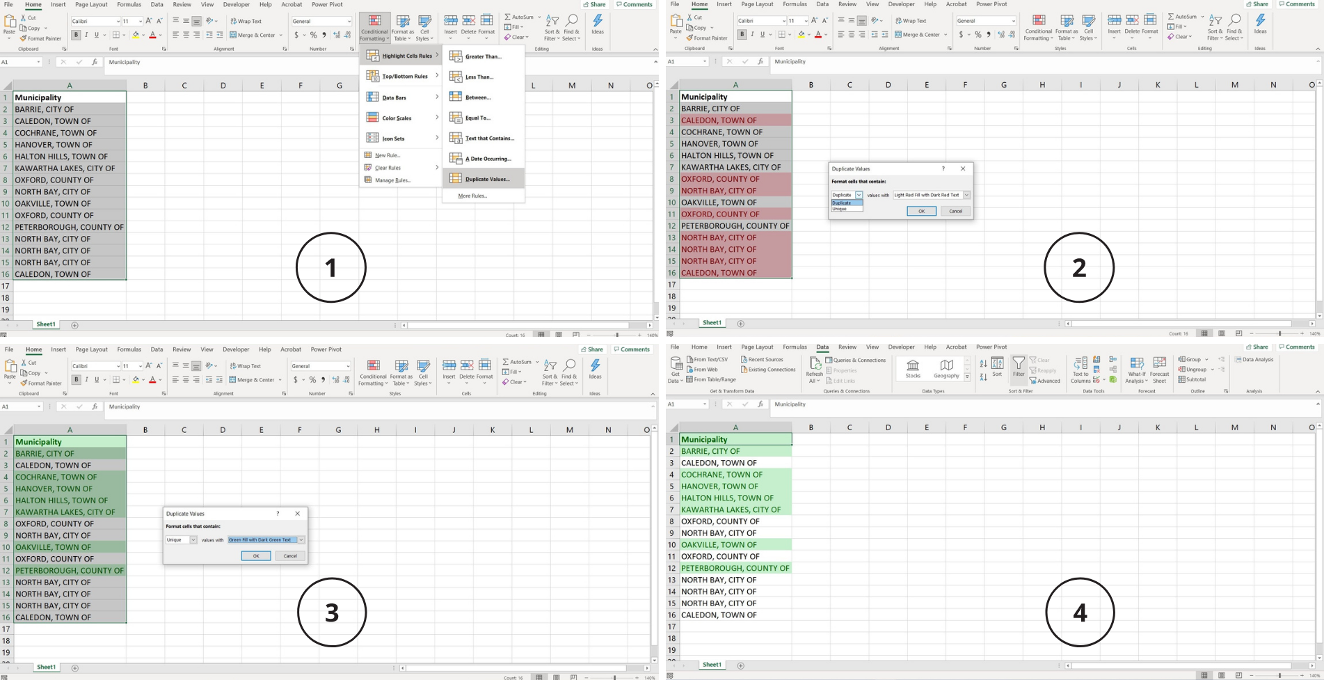
Step 1: select a list or a table where to want to highlight duplicate or unique values from
Step 2: click on the Home tab => Look for “Conditional Formatting”
Step 3: select Highlight Cells Rules from the drop-down menu and then select Duplicate Values
Step 4: the pop-up menu will ask you if you want duplicate or unique values to be highlighted and you can also select how to format those values
Step 5: click Ok

I selected unique values to be highlighted with green font and cell background. There is also a custom formatting option in that pop-up menu. Now we can see all the municipalities that were entered only once into that list. Formatting makes working with data easier. Yes, way easier. I am sure you are familiar with Excel filters, but repetition is a mother of learning.

4.    Filters
Filters is one of the most helpful tools for any excel user, particularly when you deal with hundreds and hundreds of lines of data. Let’s go back to that list of municipalities once again.
Previously we applied formatting to unique amounts. The beauty of filters is that you can filter your data by cell colour, font colour, value, text content, etc.

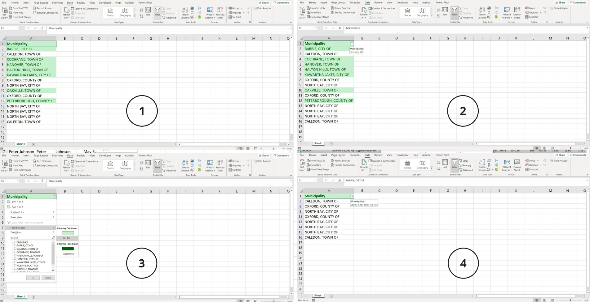
Step 1: select the heading of your table weather it has one column or multiple columns
Step 2: click on the Data tab => Look for another magical symbol, it is silo looking and it says “Filter” on it  
Step 3: after I click on it, the table header “Municipality” becomes a drop-down list (or if a table has multiple columns, they all become drop down lists; you can filter by multiple criteria at the same time). This is where you can filter cells by colour or no colour, or only select certain data points you would like to see (unselect Select All before that).
Step 4: after I clicked on the “Municipality” drop-down list, selected Filter by Colour => Filter by Cell Colour => No Fill I got a list of municipalities that were entered several times into that column.

If I were to filter by green colour I would have gotten a list of unique municipalities from the previous example. That way if you scroll through your data highlighting any key cells or rows you can easily engage a filter and get a list of only rows/cells you highlighted.

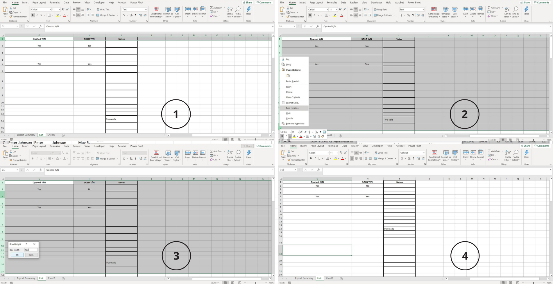
5.    Row height

Have you seen spreadsheets where all the rows are different height? This makes those spreadsheets look untidy. For an instant improvement just make row height the same for all rows, only, of course, if the data allows.

Step 1: place your cursor on a row number in a left-hand corner and highlight all the rows you would like to change the height for
Step 2: right-click while your cursor is on a row number and select Row Height. 
Step 3: enter a desired row height into the pop-up menu. Anywhere from 14.4 to 16 will make your rows look nice, but it is a personal preference
Step 4: click Ok

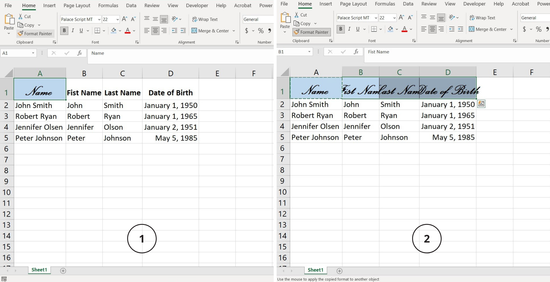
6.    Format Painter

Another undervalued hero of the Excel toolkit is Format Painter. Sometimes I spend so much time formatting one cell, picking the colour and font and then realizing that I must go through the same thing many times to make all other cells look uniform. Here’s where the Format Painter comes to save you.

Step 1: select a cell or multiple cells with format you like
Step 2: click on Home tab=> and then on Format Painter 
Step 3: double click if you would like to repeat that format on multiple cells 
Step 4: start clicking on the cells you would like to format. It is magic!

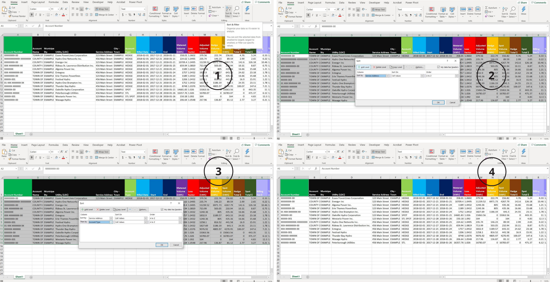
7.    Custom Sorting

Last tip on my list, but not in terms of value is Custom Sorting. When you have a table with data and you would like to sort it by several columns, this is where you cannot go wrong with Custom Sorting. In this example I have a table with data, and I want to sort it by service address and account type for convenience.

Step 1: click on Home tab=> then AZ Sort&Filter => select Custom Sort in a drop-down menu 
Step 2: in the pop-up menu specify if your table has headers, remove the check mark if it does not. In this example I do.
Step 3: in the pop-up menu I select “Service Address” as the first sorting level
Step 4: click Add Level and select “Account Type” as the second sorting level (you can drag and drop and switch levels if you desire)
Step 5: click Ok

Now our whole table is resorted.

Isn’t Excel magical?!